Training on Statistics and Data Analysis using R 👨💻
Post Graduate Students, CPEB Club, University of Ibadan
2023-08-19
About me✍️✍️✍️
I am an Agrometeorologist and Processed-Based Modeller
I am a mentor in the R4DS online learning community
I am also a active member of the TidyTuesday project
: @OluwafemOyedele 👍

My R journey (so far 👨💻👨💻👨💻️

Learning Objectives✍️✍️✍️
Installation of R and R Studio
Introduction to R and R Studio.
Data Import and Export
Data summary (Simple Descriptive analysis)
Data wrangling
Overview
By the end of this training, you should feel confident approaching data from the agricultural sector using R
We will cover virtually no statistics
-
However it is the intention that this training will leave you comfortable to:
understand/solve statistical problems using R
interpret results generated by R
Installation

Install R and R Studio)
- The first thing you need to do is download the R and R Studio software. Go to the (https://posit.co/download/rstudio-desktop/ and download the software for your operating system (Windows, Mac, or Linux).

RStudio Installation Cont.

Download Training Material from Github
Option 1: Download the zip file directly from github and then unzip it
Option 2: Run the following command below in RStudio console pane:
- You’ll now have a copy of the project created for this training on your computer.
Congratulation We are now set for the Training !!!

What is R💥💥💥

A widely used programming language for data analysis
Based on statistical programming language S (1976)
Developed by Ross Ihaka & Robert Gentleman (1995)
Very active community, with many packages
Open source, and interoperable!
If one already knows Stata or similar software, why use R?😂😂😂
R is free, so you don’t need a terminal server
R has a very large community.
R can handle virtually any data format.
Analyses done using R are reproducible
Using R makes collaboration easier.
Finding answers to questions is much simpler in R
What is R Studio ️👁️🗨️👁️🗨️👁️🗨️
![]()
Integrated Development Environment (IDE) for R that can make your life easier.
Founded by J.J. Allaire, available since 2010
RStudio can:💥💥💥
Organize your code, output, and plots.
Auto-complete code and highlight syntax.
Help view data and objects.
Enable easy integration of R code into documents with
quartoandR Markdown
Open R Studio
- We should see something like this
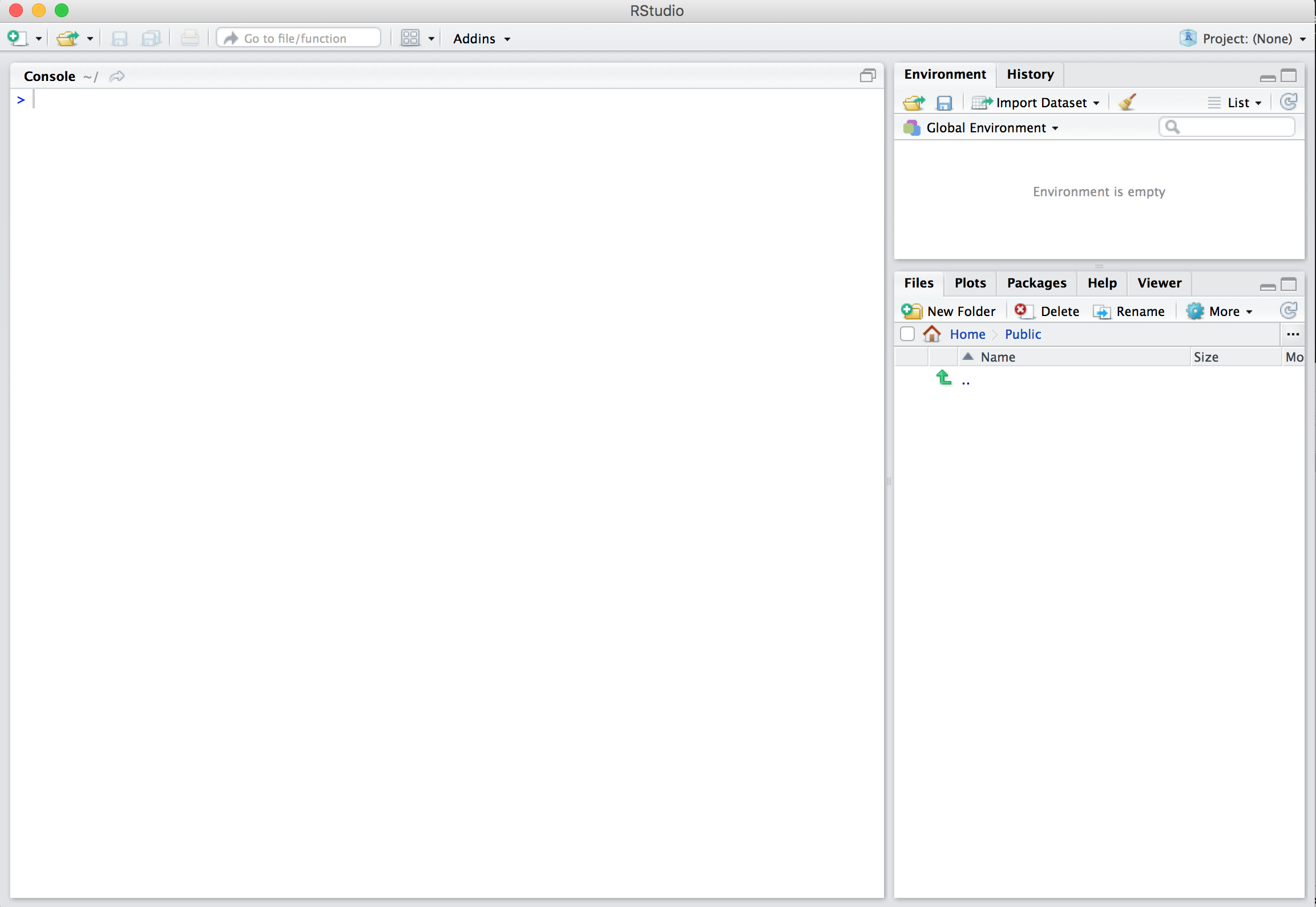
R Studio Interface

Demonstration👨💻👨💻👨💻
- Demontration on the various tabs found in R and R Studio.
Working Directly in R Console
Enter: 2 + 2
Hit return
View result
We can create new object with the assignment (
<-) operatorR is case sensitive
Your Turn
Open RStudio and try the following tasks:
Pick a number and add 2 to it
Multiply the result by 3
Subtract 6 from the result of step 2
Divide the result of step 3 by 3
What do you think
factorial(round(2.0015) + 1)will return?
Working Directories
Functions and Help
-
sqrt()is an example of afunctionin R
Creating Objects
Using Objects
R Studio Projects
RStudio projects allow you to keep a collection of files all together, including:
R scripts
Quarto and Rmarkdown files (more on those soon)
Data files
And much more!
How to Create a Project
File -> New Project
Give the project a unique name
Set the directory where you want to put the project.
Quit RStudio, Double-click .Rproj file to reopen project
Your Turn
Create a new project (doesn’t matter if it’s in a new or existing directory
Quit RStudio, double-click the .Rproj file and reopen your project
Working directory
When you start R, it associates itself with a folder (i.e, directory) on your computer:
This folder is known as your “working directory
When you save files, R will save them here
When you load files, R will look for them here
Changing the Working directory
First option: Navigate in the files pane to a new directory. Click More>Set As Working Directory
Second option: In the toolbar, go to Session>Set Working Directory>Choose Directory…
File Types in R
There are two main file types that you’ll work with:
R scripts (.R)
Text is assumed to be executable R code unless you comment it
Quarto files (.qmd)
Text is assumed to be text unless you put it in a code chunk (more on this soon)

R Scripts
- Create new script file: File -> New File -> R Script

How to Run Code
- Run the code: control + enter on Windows, command + enter on Mac keystrokes or use Run button

How to Run Code Continuation
Note that you don’t have to highlight code.
You can just hit run anywhere on line to run code.
Packages
An R package is a collection of functions, data and documentation that extends the capability of base R.
Packages add functionality that is not present in base R.
They’re where much of the power of R is found.

Packages We’ll Use

Packages We’ll Use

skimr
-
skimrprovides easy summary statistics.
Install Packages
- The syntax to install packages is as follows.
The package name must be in quotes.
Packages should be installed once per computer (i.e. once you’ve installed a package, you don’t need to do it again on the same computer).
Load Packages
- To load packages, use the following syntax:
Package names don’t need to be quoted here (though they can be).
Packages should be loaded once per session (i.e. every time you start working in R, you need to load any packages you want to use).
Your Turn
Open the project you downloaded before (it should be on your desktop)
Open the readme.md file
Install all the packages
Load the tidyverse and skimr packages using the library function
Data Science Workflow in R by (Hadley Wickham) (Continue)

Data Import
To read in a csv file into R we will use
read_csvTo read in an excel file into R we will use
read_excelTo write a csv file to disc we will use
write_csvTo write a excel file to disc we will use
write_xlsxfromwritexl package
R is Case Sensitive
Option
snake_case
camelCase
periods.in.names
Example
student_data
studentData
student.data
Data Import Practicals
Import
sorghum.xlsxinto RStudio and assigned it to an object calledsorghnum_dat.View the first 6 rows of the dataset.
View the last 6 rows of the dataset.
Data Types
Double/Numeric (e.g. 2.5)
Character (e.g. “Male”)
Logical (e.g. “TRUE and FALSE”)
Data Frames
A
data frameis a two dimensional group of R objects.Each column in a
data framecan be a different typeWe can think of a data frame as R’s equivalent to the Excel spreadsheet because it stores data in a similar format.
Creating a
data frameby hand takes a lot of typing, but we can do it with thedata.framefunction
Data Frame Example
Inspection of a Data Frame Object
Inspection of a Data Frame Object Cont.
What is tidy data?
Data that is easy to model, visualise and aggregate (i.e. works well with lm, ggplot, and dplyr)
A step along the road to clean data

The Philosophy of Tidy Data
Data can be messy or tidy. Messy data can be in a number of different ways, but tidy data is any dataset where:
Each variable is a column; each column is a variable
Each observation is a row; each row is an observation
Each value is a cell; each cell is a single value
Tidy Data Example
Making Table3 to Tidy Data
# A tibble: 6 × 4
  country      year Cases  Population
  <chr>       <dbl> <chr>  <chr>
1 Afghanistan  1999 745    19987071
2 Afghanistan  2000 2666   20595360
3 Brazil       1999 37737  172006362
4 Brazil       2000 80488  174504898
5 China        1999 212258 1272915272
6 China        2000 213766 1280428583
Data in column names
# A tibble: 6 × 79
artist track date.entered wk1 wk2 wk3 wk4 wk5 wk6 wk7 wk8
<chr> <chr> <date> <dbl> <dbl> <dbl> <dbl> <dbl> <dbl> <dbl> <dbl>
1 2 Pac Baby… 2000-02-26 87 82 72 77 87 94 99 NA
2 2Ge+her The … 2000-09-02 91 87 92 NA NA NA NA NA
3 3 Doors Do… Kryp… 2000-04-08 81 70 68 67 66 57 54 53
4 3 Doors Do… Loser 2000-10-21 76 76 72 69 67 65 55 59
5 504 Boyz Wobb… 2000-04-15 57 34 25 17 17 31 36 49
6 98^0 Give… 2000-08-19 51 39 34 26 26 19 2 2
# ℹ 68 more variables: wk9 <dbl>, wk10 <dbl>, wk11 <dbl>, wk12 <dbl>,
# wk13 <dbl>, wk14 <dbl>, wk15 <dbl>, wk16 <dbl>, wk17 <dbl>, wk18 <dbl>,
# wk19 <dbl>, wk20 <dbl>, wk21 <dbl>, wk22 <dbl>, wk23 <dbl>, wk24 <dbl>,
# wk25 <dbl>, wk26 <dbl>, wk27 <dbl>, wk28 <dbl>, wk29 <dbl>, wk30 <dbl>,
# wk31 <dbl>, wk32 <dbl>, wk33 <dbl>, wk34 <dbl>, wk35 <dbl>, wk36 <dbl>,
# wk37 <dbl>, wk38 <dbl>, wk39 <dbl>, wk40 <dbl>, wk41 <dbl>, wk42 <dbl>,
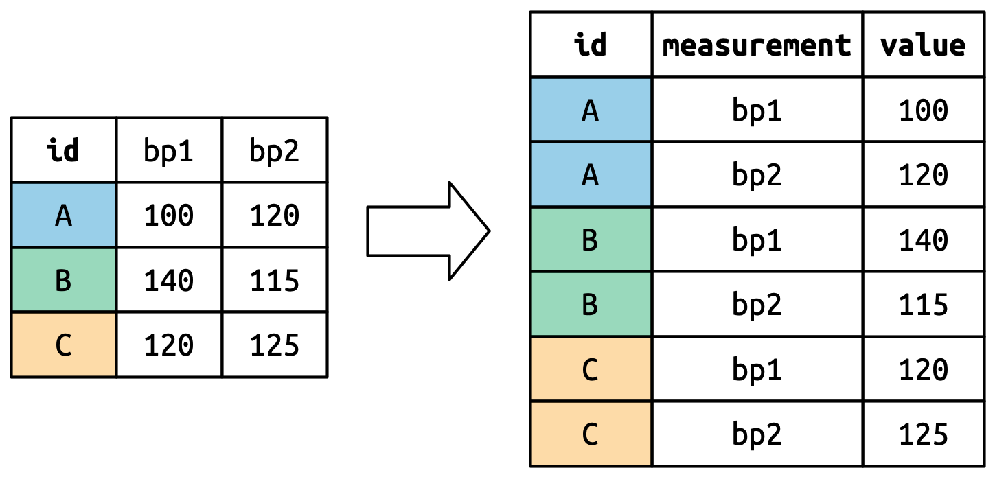
# wk43 <dbl>, wk44 <dbl>, wk45 <dbl>, wk46 <dbl>, wk47 <dbl>, wk48 <dbl>, …Pivot Longer Function from Tidyr
library(dplyr)
library(tidyr)
billboard %>%
  pivot_longer(cols = starts_with('wk'),
               names_to = 'Week',
               values_to = 'Rank')
# A tibble: 24,092 × 5
artist track date.entered Week Rank
<chr> <chr> <date> <chr> <dbl>
1 2 Pac Baby Don't Cry (Keep... 2000-02-26 wk1 87
2 2 Pac Baby Don't Cry (Keep... 2000-02-26 wk2 82
3 2 Pac Baby Don't Cry (Keep... 2000-02-26 wk3 72
4 2 Pac Baby Don't Cry (Keep... 2000-02-26 wk4 77
5 2 Pac Baby Don't Cry (Keep... 2000-02-26 wk5 87
6 2 Pac Baby Don't Cry (Keep... 2000-02-26 wk6 94
7 2 Pac Baby Don't Cry (Keep... 2000-02-26 wk7 99
8 2 Pac Baby Don't Cry (Keep... 2000-02-26 wk8 NA
9 2 Pac Baby Don't Cry (Keep... 2000-02-26 wk9 NA
10 2 Pac Baby Don't Cry (Keep... 2000-02-26 wk10 NA
# ℹ 24,082 more rowsHow to Drop Missing Values
library(dplyr)
library(tidyr)
billboard |>
  pivot_longer(
    cols = starts_with("wk"),
    names_to = "week",
    values_to = "rank",
    values_drop_na = TRUE
  )
# A tibble: 5,307 × 5
artist track date.entered week rank
<chr> <chr> <date> <chr> <dbl>
1 2 Pac Baby Don't Cry (Keep... 2000-02-26 wk1 87
2 2 Pac Baby Don't Cry (Keep... 2000-02-26 wk2 82
3 2 Pac Baby Don't Cry (Keep... 2000-02-26 wk3 72
4 2 Pac Baby Don't Cry (Keep... 2000-02-26 wk4 77
5 2 Pac Baby Don't Cry (Keep... 2000-02-26 wk5 87
6 2 Pac Baby Don't Cry (Keep... 2000-02-26 wk6 94
7 2 Pac Baby Don't Cry (Keep... 2000-02-26 wk7 99
8 2Ge+her The Hardest Part Of ... 2000-09-02 wk1 91
9 2Ge+her The Hardest Part Of ... 2000-09-02 wk2 87
10 2Ge+her The Hardest Part Of ... 2000-09-02 wk3 92
# ℹ 5,297 more rowsHow Does Pivot Longer Works
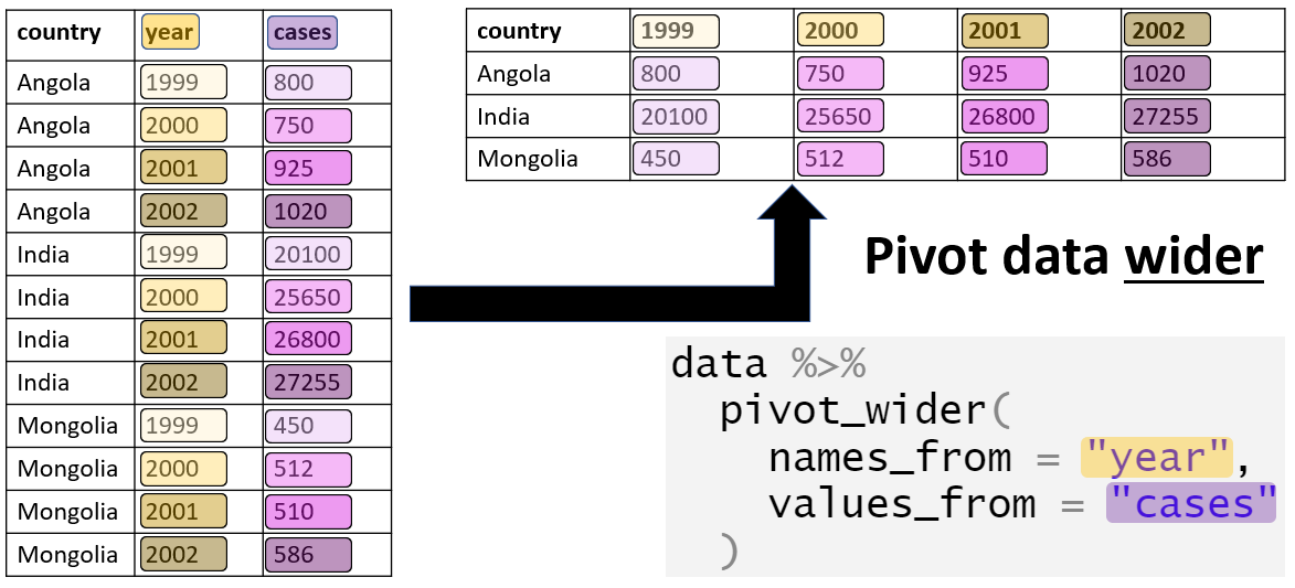
Pivot Wider
Pivot Wider Example
How Does Pivot Wider Works
Summary Statistics of the dataset
── Data Summary ────────────────────────
                           Values
Name                       iris
Number of rows             150
Number of columns          5
_______________________
Column type frequency:
  factor                   1
  numeric                  4
________________________
Group variables            None

── Variable type: factor ───────────────────────────────────────────────────────
  skim_variable n_missing complete_rate ordered n_unique
1 Species               0             1 FALSE          3
  top_counts
1 set: 50, ver: 50, vir: 50

── Variable type: numeric ──────────────────────────────────────────────────────
  skim_variable n_missing complete_rate mean    sd  p0 p25  p50 p75 p100 hist
1 Sepal.Length          0             1 5.84 0.828 4.3 5.1 5.8  6.4  7.9 ▆▇▇▅▂
2 Sepal.Width           0             1 3.06 0.436 2   2.8 3    3.3  4.4 ▁▆▇▂▁
3 Petal.Length          0             1 3.76 1.77  1   1.6 4.35 5.1  6.9 ▇▁▆▇▂
4 Petal.Width           0             1 1.20 0.762 0.1 0.3 1.3  1.8  2.5 ▇▁▇▅▃
Data Transformation
There are five key dplyr functions in tidyverse to solve most of data manipulation challenges:
Pick observations by their values –
filter()Reorder (sort) the rows –
arrange()Pick variables by their names –
select()Create new variables with functions of existing variables –
mutate()Collapse many values down to a summary –
summarize()
Data Transformation: Filter
filter()allows to subset observations based on their valuesfilter(data, expressions)The first argument is the name of the data frame The second and subsequent arguments are the expressions that filter the data frame
To use filter effectively we need to make proper use of the comparison operators i.e. (
>,>=,<,<=,!=and==)
Data Transformation: Filter
  env rep gen  yield
1  E1  R1 G01 139.82
2  E1  R1 G02 182.52
3  E1  R1 G03 171.71
4  E1  R1 G04 200.49
5  E1  R1 G05 157.23
6  E1  R1 G06 177.22
7 E1 R1 G07 55.36
8 E1 R1 G08 89.54
9 E1 R1 G09 296.50
10 E1 R1 G10 312.21
11 E1 R1 G11 189.00
12 E1 R1 G12 191.90
13 E1 R1 G13 76.46
14 E1 R1 G14 111.02
15 E1 R1 G15 22.30
16 E1 R1 G16 208.14
17 E1 R1 G17 19.81
18 E1 R1 G18 208.63
19 E1 R2 G01 141.26
20 E1 R2 G02 182.52
21 E1 R2 G03 160.97
22 E1 R2 G04 164.43
23 E1 R2 G05 157.23
24 E1 R2 G06 209.38
25 E1 R2 G07 36.59
26 E1 R2 G08 186.04
27 E1 R2 G09 117.47
28 E1 R2 G10 261.03
29 E1 R2 G11 177.81
30 E1 R2 G12 136.19
31 E1 R2 G13 102.65
32 E1 R2 G14 113.56
33 E1 R2 G15 34.50
34 E1 R2 G16 171.96
35 E1 R2 G17 19.81
36 E1 R2 G18 174.48
37 E1 R3 G01 126.72
38 E1 R3 G02 182.52
39 E1 R3 G03 138.15
40 E1 R3 G04 143.66
41 E1 R3 G05 157.23
42 E1 R3 G06 97.89
43 E1 R3 G07 17.81
44 E1 R3 G08 105.88
45 E1 R3 G09 190.61
46 E1 R3 G10 286.62
47 E1 R3 G11 178.94
48 E1 R3 G12 158.15
49 E1 R3 G13 109.12
50 E1 R3 G14 100.63
51 E1 R3 G15 22.30
52 E1 R3 G16 187.13
53 E1 R3 G17 19.81
54 E1 R3 G18 192.81
55 E1 R4 G01 114.52
56 E1 R4 G02 182.52
57 E1 R4 G03 166.40
58 E1 R4 G04 233.68
59 E1 R4 G05 157.23
60 E1 R4 G06 173.92
61 E1 R4 G07 36.59
62 E1 R4 G08 109.22
63 E1 R4 G09 337.58
64 E1 R4 G10 286.62
65 E1 R4 G11 162.52
66 E1 R4 G12 143.02
67 E1 R4 G13 97.21
68 E1 R4 G14 77.32
69 E1 R4 G15 10.17
70 E1 R4 G16 185.20
71 E1 R4 G17 19.81
72 E1 R4 G18 122.02Data Transformation: Filter
- What does the following command do?
   env rep gen  yield
1   E1  R1 G01 139.82
2   E1  R1 G02 182.52
3   E1  R1 G03 171.71
4   E1  R1 G04 200.49
5   E1  R1 G05 157.23
6   E1  R1 G06 177.22
7   E1  R1 G07  55.36
8   E1  R1 G08  89.54
9   E1  R1 G09 296.50
10  E1  R1 G10 312.21
11  E1  R1 G11 189.00
12  E1  R1 G12 191.90
13  E1  R1 G13  76.46
14  E1  R1 G14 111.02
15  E1  R1 G15  22.30
16  E1  R1 G16 208.14
17  E1  R1 G17  19.81
18  E1  R1 G18 208.63
19  E1  R2 G01 141.26
20  E1  R2 G02 182.52
21  E1  R2 G03 160.97
22  E1  R2 G04 164.43
23  E1  R2 G05 157.23
24  E1  R2 G06 209.38
25  E1  R2 G07  36.59
26  E1  R2 G08 186.04
27  E1  R2 G09 117.47
28  E1  R2 G10 261.03
29  E1  R2 G11 177.81
30  E1  R2 G12 136.19
31  E1  R2 G13 102.65
32  E1  R2 G14 113.56
33  E1  R2 G15  34.50
34  E1  R2 G16 171.96
35  E1  R2 G17  19.81
36  E1  R2 G18 174.48
37  E1  R3 G01 126.72
38  E1  R3 G02 182.52
39  E1  R3 G03 138.15
40  E1  R3 G04 143.66
41  E1  R3 G05 157.23
42  E1  R3 G06  97.89
43  E1  R3 G07  17.81
44  E1  R3 G08 105.88
45  E1  R3 G09 190.61
46  E1  R3 G10 286.62
47  E1  R3 G11 178.94
48  E1  R3 G12 158.15
49  E1  R3 G13 109.12
50  E1  R3 G14 100.63
51  E1  R3 G15  22.30
52  E1  R3 G16 187.13
53  E1  R3 G17  19.81
54  E1  R3 G18 192.81
55  E1  R4 G01 114.52
56  E1  R4 G02 182.52
57  E1  R4 G03 166.40
58  E1  R4 G04 233.68
59  E1  R4 G05 157.23
60  E1  R4 G06 173.92
61  E1  R4 G07  36.59
62  E1  R4 G08 109.22
63  E1  R4 G09 337.58
64  E1  R4 G10 286.62
65  E1  R4 G11 162.52
66  E1  R4 G12 143.02
67  E1  R4 G13  97.21
68  E1  R4 G14  77.32
69  E1  R4 G15  10.17
70  E1  R4 G16 185.20
71  E1  R4 G17  19.81
72  E1  R4 G18 122.02
73 E2 R1 G01 401.71
74 E2 R1 G02 296.22
75 E2 R1 G03 180.31
76 E2 R1 G04 102.44
77 E2 R1 G05 174.77
78 E2 R1 G06 101.79
79 E2 R1 G07 342.70
80 E2 R1 G08 635.42
81 E2 R1 G09 601.30
82 E2 R1 G10 268.96
83 E2 R1 G11 181.88
84 E2 R1 G12 333.85
85 E2 R1 G13 473.24
86 E2 R1 G14 423.43
87 E2 R1 G15 227.89
88 E2 R1 G16 399.58
89 E2 R1 G17 312.58
90 E2 R1 G18 300.55
91 E2 R2 G01 210.38
92 E2 R2 G02 375.53
93 E2 R2 G03 51.14
94 E2 R2 G04 87.83
95 E2 R2 G05 38.22
96 E2 R2 G06 59.34
97 E2 R2 G07 60.21
98 E2 R2 G08 470.73
99 E2 R2 G09 490.42
100 E2 R2 G10 169.50
101 E2 R2 G11 367.92
102 E2 R2 G12 405.51
103 E2 R2 G13 591.95
104 E2 R2 G14 226.56
105 E2 R2 G15 555.83
106 E2 R2 G16 267.66
107 E2 R2 G17 293.45
108 E2 R2 G18 249.79
109 E2 R3 G01 166.95
110 E2 R3 G02 337.11
111 E2 R3 G03 385.30
112 E2 R3 G04 148.35
113 E2 R3 G05 104.99
114 E2 R3 G06 104.79
115 E2 R3 G07 84.98
116 E2 R3 G08 238.12
117 E2 R3 G09 375.67
118 E2 R3 G10 243.75
119 E2 R3 G11 607.38
120 E2 R3 G12 530.08
121 E2 R3 G13 490.56
122 E2 R3 G14 345.96
123 E2 R3 G15 365.30
124 E2 R3 G16 182.14
125 E2 R3 G17 35.40
126 E2 R3 G18 266.65
127 E2 R4 G01 192.17
128 E2 R4 G02 314.83
129 E2 R4 G03 231.17
130 E2 R4 G04 176.17
131 E2 R4 G05 102.79
132 E2 R4 G06 404.35
133 E2 R4 G07 266.55
134 E2 R4 G08 585.90
135 E2 R4 G09 291.40
136 E2 R4 G10 103.68
137 E2 R4 G11 257.85
138 E2 R4 G12 754.33
139 E2 R4 G13 1018.29
140 E2 R4 G14 299.71
141 E2 R4 G15 614.77
142 E2 R4 G16 225.18
143 E2 R4 G17 532.77
144 E2 R4 G18 223.92Data Transformation: Filter Practical 5 minutes
import
mtcars.csvdata into RStudiofilterformpg<20andgear==4
Data Transformation: Arrange
-
arrange()changes the order of the rows (sorting): it takes a data frame and a set of column names to order by
                     mpg cyl  disp  hp drat    wt  qsec vs am gear carb
Cadillac Fleetwood  10.4   8 472.0 205 2.93 5.250 17.98  0  0    3    4
Lincoln Continental 10.4   8 460.0 215 3.00 5.424 17.82  0  0    3    4
Camaro Z28          13.3   8 350.0 245 3.73 3.840 15.41  0  0    3    4
Duster 360          14.3   8 360.0 245 3.21 3.570 15.84  0  0    3    4
Chrysler Imperial   14.7   8 440.0 230 3.23 5.345 17.42  0  0    3    4
Maserati Bora       15.0   8 301.0 335 3.54 3.570 14.60  0  1    5    8
Merc 450SLC         15.2   8 275.8 180 3.07 3.780 18.00  0  0    3    3
AMC Javelin         15.2   8 304.0 150 3.15 3.435 17.30  0  0    3    2
Dodge Challenger    15.5   8 318.0 150 2.76 3.520 16.87  0  0    3    2
Ford Pantera L      15.8   8 351.0 264 4.22 3.170 14.50  0  1    5    4
Data Transformation: Arrange
We can use the function desc() to re-order by a column in descending order
                     mpg cyl  disp  hp drat    wt  qsec vs am gear carb
Toyota Corolla      33.9   4  71.1  65 4.22 1.835 19.90  1  1    4    1
Fiat 128            32.4   4  78.7  66 4.08 2.200 19.47  1  1    4    1
Honda Civic         30.4   4  75.7  52 4.93 1.615 18.52  1  1    4    2
Lotus Europa        30.4   4  95.1 113 3.77 1.513 16.90  1  1    5    2
Fiat X1-9           27.3   4  79.0  66 4.08 1.935 18.90  1  1    4    1
Porsche 914-2       26.0   4 120.3  91 4.43 2.140 16.70  0  1    5    2
Merc 240D           24.4   4 146.7  62 3.69 3.190 20.00  1  0    4    2
Datsun 710          22.8   4 108.0  93 3.85 2.320 18.61  1  1    4    1
Merc 230            22.8   4 140.8  95 3.92 3.150 22.90  1  0    4    2
Toyota Corona       21.5   4 120.1  97 3.70 2.465 20.01  1  0    3    1
Hornet 4 Drive      21.4   6 258.0 110 3.08 3.215 19.44  1  0    3    1
Volvo 142E          21.4   4 121.0 109 4.11 2.780 18.60  1  1    4    2
Mazda RX4           21.0   6 160.0 110 3.90 2.620 16.46  0  1    4    4
Mazda RX4 Wag       21.0   6 160.0 110 3.90 2.875 17.02  0  1    4    4
Ferrari Dino        19.7   6 145.0 175 3.62 2.770 15.50  0  1    5    6
Merc 280            19.2   6 167.6 123 3.92 3.440 18.30  1  0    4    4
Pontiac Firebird    19.2   8 400.0 175 3.08 3.845 17.05  0  0    3    2
Hornet Sportabout   18.7   8 360.0 175 3.15 3.440 17.02  0  0    3    2
Valiant             18.1   6 225.0 105 2.76 3.460 20.22  1  0    3    1
Merc 280C           17.8   6 167.6 123 3.92 3.440 18.90  1  0    4    4
Merc 450SL          17.3   8 275.8 180 3.07 3.730 17.60  0  0    3    3
Merc 450SE          16.4   8 275.8 180 3.07 4.070 17.40  0  0    3    3
Ford Pantera L      15.8   8 351.0 264 4.22 3.170 14.50  0  1    5    4
Dodge Challenger    15.5   8 318.0 150 2.76 3.520 16.87  0  0    3    2
Merc 450SLC         15.2   8 275.8 180 3.07 3.780 18.00  0  0    3    3
AMC Javelin         15.2   8 304.0 150 3.15 3.435 17.30  0  0    3    2
Maserati Bora       15.0   8 301.0 335 3.54 3.570 14.60  0  1    5    8
Chrysler Imperial   14.7   8 440.0 230 3.23 5.345 17.42  0  0    3    4
Duster 360          14.3   8 360.0 245 3.21 3.570 15.84  0  0    3    4
Camaro Z28          13.3   8 350.0 245 3.73 3.840 15.41  0  0    3    4
Cadillac Fleetwood  10.4   8 472.0 205 2.93 5.250 17.98  0  0    3    4
Lincoln Continental 10.4   8 460.0 215 3.00 5.424 17.82  0  0    3    4
Data Transformation: Select
Select help us to pick variable by their position or name in a
dataframe.We can also used other
selecthelpers function likestart_with,end_with,containsandeverything
                     mpg cyl  disp
Mazda RX4           21.0   6 160.0
Mazda RX4 Wag       21.0   6 160.0
Datsun 710          22.8   4 108.0
Hornet 4 Drive      21.4   6 258.0
Hornet Sportabout   18.7   8 360.0
Valiant             18.1   6 225.0
Duster 360          14.3   8 360.0
Merc 240D           24.4   4 146.7
Merc 230            22.8   4 140.8
Merc 280            19.2   6 167.6
Merc 280C           17.8   6 167.6
Merc 450SE          16.4   8 275.8
Merc 450SL          17.3   8 275.8
Merc 450SLC         15.2   8 275.8
Cadillac Fleetwood  10.4   8 472.0
Lincoln Continental 10.4   8 460.0
Chrysler Imperial   14.7   8 440.0
Fiat 128            32.4   4  78.7
Honda Civic         30.4   4  75.7
Toyota Corolla      33.9   4  71.1
Toyota Corona       21.5   4 120.1
Dodge Challenger    15.5   8 318.0
AMC Javelin         15.2   8 304.0
Camaro Z28          13.3   8 350.0
Pontiac Firebird    19.2   8 400.0
Fiat X1-9           27.3   4  79.0
Porsche 914-2       26.0   4 120.3
Lotus Europa        30.4   4  95.1
Ford Pantera L      15.8   8 351.0
Ferrari Dino        19.7   6 145.0
Maserati Bora       15.0   8 301.0
Volvo 142E          21.4   4 121.0
Data Transformation: Mutate
- We can add new columns that are functions of existing columns with
mutate()which always adds new columns at the end of the dataset
                   mpg cyl  disp  hp drat    wt  qsec vs am gear carb mpg_trans
Mazda RX4         21.0   6 160.0 110 3.90 2.620 16.46  0  1    4    4  1.322219
Mazda RX4 Wag     21.0   6 160.0 110 3.90 2.875 17.02  0  1    4    4  1.322219
Datsun 710        22.8   4 108.0  93 3.85 2.320 18.61  1  1    4    1  1.357935
Hornet 4 Drive    21.4   6 258.0 110 3.08 3.215 19.44  1  0    3    1  1.330414
Hornet Sportabout 18.7   8 360.0 175 3.15 3.440 17.02  0  0    3    2  1.271842
Valiant           18.1   6 225.0 105 2.76 3.460 20.22  1  0    3    1  1.257679
Duster 360        14.3   8 360.0 245 3.21 3.570 15.84  0  0    3    4  1.155336
Merc 240D         24.4   4 146.7  62 3.69 3.190 20.00  1  0    4    2  1.387390
Merc 230          22.8   4 140.8  95 3.92 3.150 22.90  1  0    4    2  1.357935
Merc 280          19.2   6 167.6 123 3.92 3.440 18.30  1  0    4    4  1.283301
Data Transformation: Summaries
-
summarize()collapses a data frame to a single or few row(s)
  mpg_mean
1 20.09062-
summarize()is useful withgroup_by()
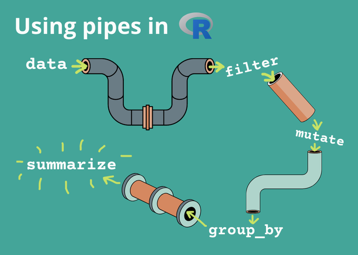
Data Transformation: The pipe %>%
The pipe help us to combine multiple operations together.
The pipe makes code easy to read.
How to use Pipes to Clean up your R Code
Data Transformation: Count
Data Wrangling: Practical
Import
sorghum.xlsxto R and save to an object named example03How many observations do we have per environment?
How many
environment?genotypes?Display the list of locations and the list ofgenotypes respectively?Display the data where the
yield was less than 150?Select
env,gen,yield, to be saved in a new objectexample03.shortand create a new variablemean_yieldby by computing the mean of theyield.
Summary
filter: pick rows matching criteria
select: pick columns by name
arrange: reorder rows
mutate: add new variables
summarise: reduce variables to values
Getting Help
- We can use the ? to get help about anything we are confused about in R.
Tidyverse Website
 (https://www.tidyverse.org/)
Package Vignettes
 (https://cran.r-project.org/web/packages/skimr/vignettes/Using_skimr.html)
 (https://twitter.com/search?q=%23rstats)
R for Data Science Community

 (https://twitter.com/ekaleedmiston/status/1081221822186696706)
Finding more functions and packages
Rseek to look for help
R Cheat Sheet
Chat GPT

Resources to Learn More
QUESTIONS?

Comments